Data Collection
Air Photos
Stereo pairs of scanned air photos were ordered for the year 2005 (Table 1) and TRIM data for the year 2003 and at a 1:20 000 resolution was acquired for the area from the GeoBC website. The air photos were imported into ArcGIS and georeferenced to the TRIM data using distinct features in the landscape such as rock knobs and deeply incised valleys as control points. After georeferencing, the air photos were used to delineate areas on the outwash plain that contained similar types of deposits, which from now on will be referred to as sediment polygons (Fig. 1). The sediment polygons were delineated based on differences in colours and texture of deposits, breaks in slope, and variations in vegetation density across the outwash plain. Each sediment polygon was then assigned a numerical ID and if there were any small scale variations within the polygons, it was subdivided and those subpolygons were given a letter (Fig 2 in Results). As some of the spatial analyses done in this study required points rather than areas as input layers, a layer comprised of points representing each of the polygon centroids was created from the sediment polygon layer.
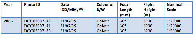
Table 1. Air photos used in the GIS analysis of Bridge Glacier
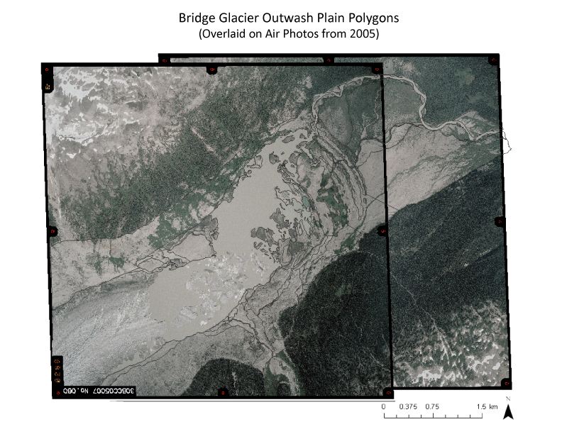
Figure 1. Delineation of sediment polygons based on air photo analysis and field observations
Field Work
Fieldwork was conducted at Bridge Glacier during three trips throughout the summer of 2011. The aims of the fieldwork were to compare the assignment of sediment polygons based on air photos to on-site observations and to collect data about sediments and vegetation from each polygon. Since it is difficult to take samples from all parts of every polygon, a representative site within each of the polygon was chosen from which to collect the necessary data. The primary variables examined in this project are found in Table 2.
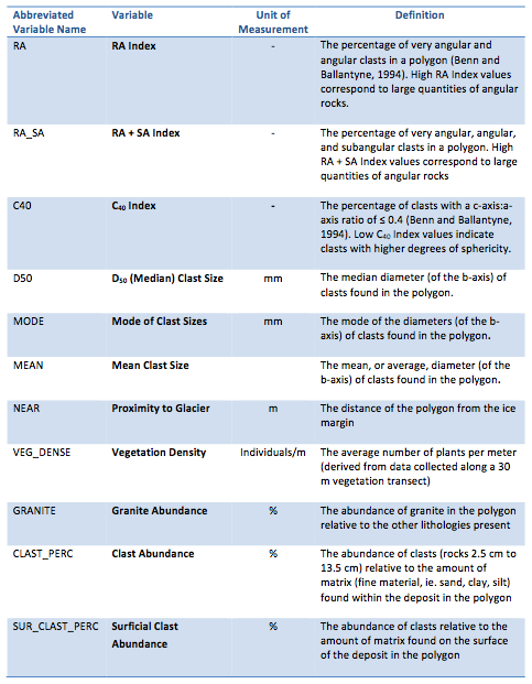
Table 2. List of variables used in this project
GIS Analysis
Once the polygons were delineated from the georeferenced air photos and the data was collected from the field, the data was entered into the attribute table of the sediment polygon layer in ArcGIS. After the spatial and attribute data was linked, it was then possible to conduct a series of spatial analysis on the data. However, prior to conducting the GIS analyses, the proglacial area was divided into six different areas based on their location and/or the deposits types within the area (Fig. 3). These were used during the analysis of the results to examine patterns of within and between these areas. The types of spatial analyses used in this project are outlined below:
Spatial Distribution
To examine the distribution of different variables within the proglacial area, a set of maps were made that displayed data that had been found for each of the different variables across the area. The first distribution map that was created was one that depicted the distribution of deposit types across the proglacial areas (Fig. 4). This map was used to look for patterns within the distribution types, such as areas that may have been deposited at the same time. This map was also used as a reference when examining the results of the different analyses in order to understand the relationship between results and the types of deposits present. Distribution maps and histograms were then created for several of the variables (Fig. 5 to 13). This set of maps was then used to look for patterns of high and low values of each of the variables across the proglacial area.
Trend Surface Analysis
Trend surfaces are created using interpolation methods which result in a smooth surface layer that represents gradual trends over the area of interest. For this project a trend surface was created for five of the variables. As trend surfaces are based on an inputted polynomial order value, ranging from 1 to 13, it is important to know which polynomial order will give the best trend surface given the characteristics of the data. To find which order of polygon to use in the trend surface analysis of the data, four maps of the variable "D50" were created using one to four orders of polynomials (Fig. 14 to 17). The resulting maps were then visually assessed in order to determine which order of polynomial produced a map with highest level of detail.
The third order polynomial was found to give the highest level of detail given the data, so trend surface maps were created for the rest of the variables using a third order polynomial as the input (Fig. 18 to 21). The resulting maps were then analysed in order to determine where the trend surface showed lower and higher values for each of the variables.
Hotspot Analysis
By calculating the Getis-Ord Gi* statistic for each feature in a dataset, the hot spot analysis tool identifies spatial clusters of high values, hot spots, and clusters of low values, cold spots. In order for a given sediment polygon, in this case, to be found as a statistically significant hot spot, the polygon itself must have a high value as well as be surrounded by other features with high values as well. This type of analysis was conducted on five variables in order to determine if there were any areas in the proglacial area where the high or low values of given variables were more aggregated. The results from this analysis can be found in Figures 21 to 25.
Ordinary Least Squares Analysis
Ordinary least squares (OLS) is a type of linear regression that is used to examine the relationship between a dependent variable and a response variable. In a regression the ability of the dependent variable to predict the response variable is quantified and residual values, which are the unexplained portion of the dependant variable, are calculated. In the case of a spatial OLS analysis, these resulting residual values, which correspond to different sediment polygons, can be mapped. Positive residual values indicate that the value of the response variable in that given area is higher than would be predicted by the OLS model whereas negative residual values indicate that the value of the response variable is lower.
For this study, five OLS analyses were run in order to examine the extent that changes in one affected changes in the another (Table 3). The residuals of each of these analyses were mapped and polygon/areas that has either extreme high or low values were noted (Figures 26 to 31). In addition to the map, a scatterplot of the two variables and the regression line was created in order to clearly see how the values were distributed and the correlation between them. Although OLS analyses are not supposed to be run on variables that have a statistically significant level of spatial autocorrelation (see next section for a definition) as this makes the results of the OLS model unreliable. One other OLS analysis was conducted in order to examine what the effects on the results using one or more spatially autocorrelated variables had, an OLS analysis was conducted using the variables "Proximity to Glacier" and "Vegetation Density", both of which are spatially autocorrelated, and the results were examined.
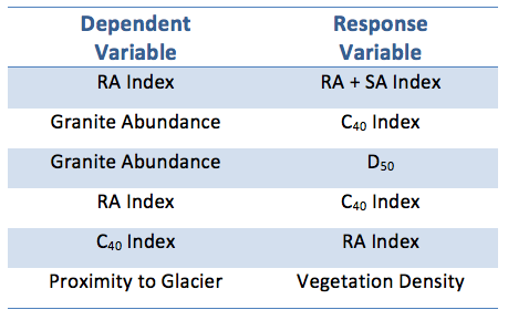
Table 3. Summary of the variables used in ordinary least squares analyses
Spatial Autocorrelation
In ArcGIS the type of spatial autocorrelation done is the calculation of Moran's Index, which evaluates whether a variable is either clustered, dispersed or found randomly across a given area by calculating a value called Moran's I. The null hypothesis of a spatial autocorrelation analysis is that the values of a given variable are randomly dispersed over the area. If the spatial distribution of an attribute is found to be significantly significant, a positive Moran's I indicates a tendency towards clustering while a negative value indicates dispersion.
In this study, spatial autocorrelations were done on two sets of data, the variables that were mapped for the spatial distribution analysis, and the residuals of the OLS analysis. Spatial autocorrelation analyses were done on the individual variables in order to better understand their distribution in the proglacial area an in order to make sure that they could properly be used in the OLS analysis. Evaluating whether the residuals of the OLS analysis are spatially autocorrelated gives further insight into the spatial trends of variables by highlighting where areas of "abnormal" values may occur. If a given variable was found to have a statistically significant Moran's I, the distribution map of that variable was examined to see where there were clusters of high/low values.
