Spatial Autocorrelation
The results from the spatial autocorrelation results are best understood in conjunction with the distribution and the OLS maps due to the fact that the analysis itself does not give mappable results. Consequently, examining the distribution of statistically significant results from the spatial autocorrelation analysis with their respective distribution maps helps to give some spatial dimension to the findings.
Individual Variables
Out of all of the variables that the spatial autocorrelation analysis was conducted on, the "vegetation density" and "proximity to the glacier" variables, were found to be statistically significantly spatially autocorrelated. Based on the fact that the distribution of vegetation density values was found have a positive Moran's I value, this variable was found to be clustered over the proglacial area. When the spatial distribution map of vegetation density is examined (Fig. 12), it is possible to see that there is a concentration of low vegetation density values in the main valley glacial deposits right next to the lake and a concentration of high vegetation density values in the South Creek tributary valley. Similarly to vegetation density, the "proximity to the glacier" variable was found to be clustered as it had a positive Moran's I value. The fact that this variable was found to be spatially autocorrelated is very predictable due to the fact that polygons that are close to the glacier terminus will have low values while those that are far away will have high values. Due to this obvious distribution of "proximity to the glacier" values, it is not included in the results table.
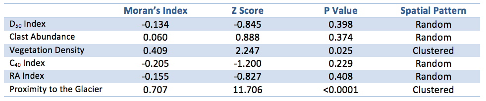
Table 6. Results from spatial autocorrelation of individual varibles
Ordinary Least Squares Residuals
Several of the results from the OLS analyses were found to be spatially autocorrelated. The OLS analysis between the RA index (as the dependent variable) and the C40 index was found to have residual values that were clustered over the proglacial area, however, when the residual map is visually examined (Fig 25a) it is difficult to see many areas where there is clustering that is occurring. Only one distinct area, the north shore deposits, seems to have a significant clustering of positive residual values. This lack of distinct clustering may be due to the the fact that the P value for this spatial autocorrelation analysis was found to be only 0.055, which is very close to the significance value of 0.05, above which results are not classified as statistically significant.
The OLS residuals from the analysis of RA index (as the dependant variable) and the RA + SA index also displayed clustering according to the spatial autocorrelation analysis. Examining the OLS results map, the clustering of residual values can be most distinctly seen within the north shore polygons, where there are several positive residual values located, and in the South Creek tributary values, where there are several polygons with negative residual values (Fig 26a).
As would be predicted by the fact that both proximity to glacier and vegetation density are spatially autocorrelated, the residuals of their OLS analysis are also autocorrelated. A trend from low residual values in close proximity of the glacier to high residual values further away from the terminus is clearly visible on the OLS results map (Fig 29a).
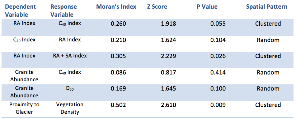
Table 7. Results from spatial autocorrelation of OLS residuals
