Ordinary Least Squares Analysis
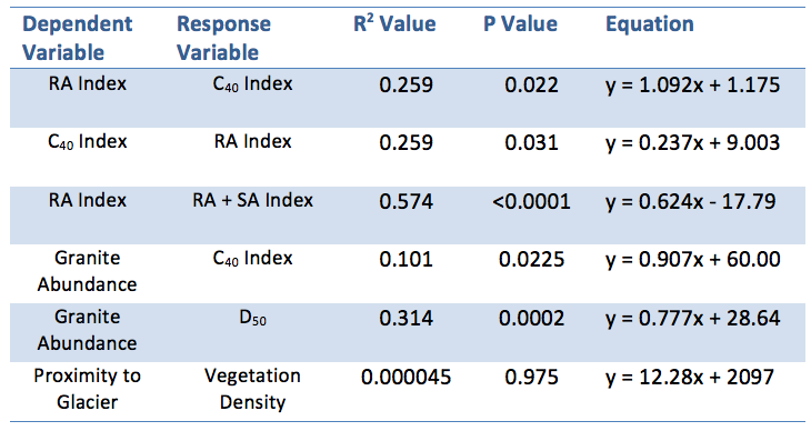
Table 5. Results from OLS analysis
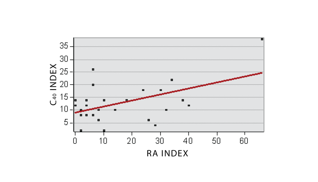
The Relationship Between the RA Index and the C40 Index
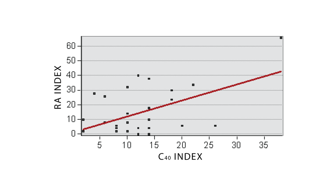
In most papers that examine clast form using the covariance of the C40 index and the RA index, the RA index is generally graphed on the y-axis while the C40 index is found on the x-axis. In a correlation test, which is what is usually conducted on these variables, the placement of a given variable on an axis does not make difference because it is the relationship of the two variables that is being examined. Conversely, during a regression analysis, such as Ordinary Least Squares (OLS) analysis, the axis chosen for a given variable does make a difference because a regression analysis is looking at the ability of one variable (the one located on the x-axis) to predict the other (the one located on the x-axis). As this study was using regression analysis as opposed to correlation to look at the relationship between the C40 Index and the RA Index, the OLS was done twice for these two variables so that both could have the chance to be the explanatory variable.
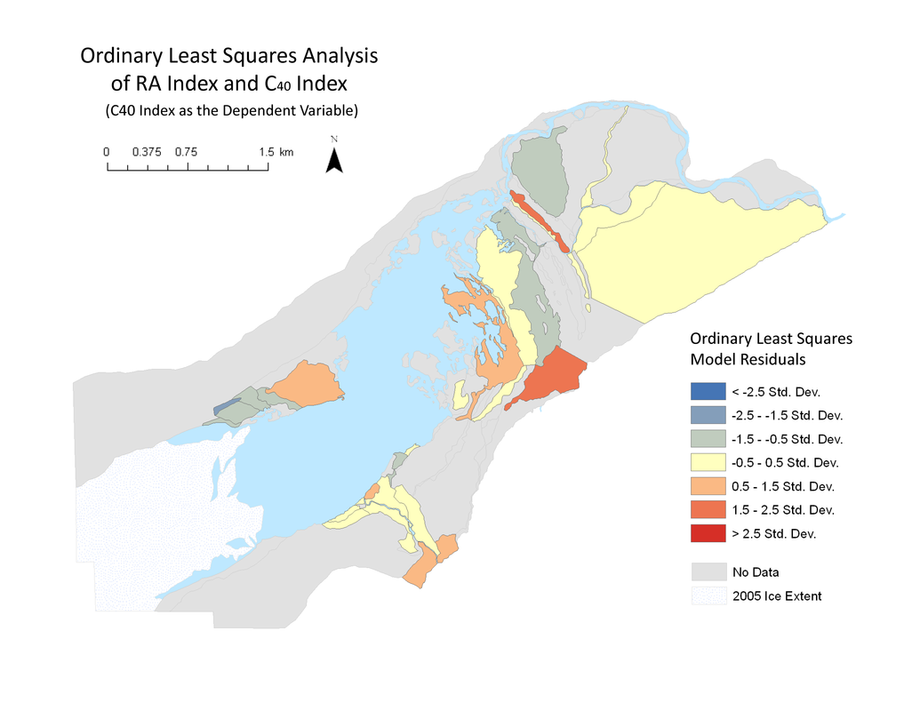
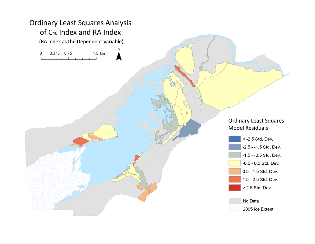
The comparison between the two resulting maps is very interesting: there are some polygons that have the same residual values for both of the analyses, some that change from a positive residual to a negative residual, and vice versa. The most notable changes from a positive residual when the C40 index is the dependent variable to a negative residual when the RA index is are the polygon at the mouth of the main spillway (polygon 19A proximal) and the ICD next to the lake in the main valley (polygon 16). The opposite is true (a switch from negative to positive) for the fluvially reworked deposits on the north side (polygon 2). The polygons that maintain the same residual values in both of the maps include the large moraine in the South Creek tributary valley (polygon 34) and the main spillway outwash plain (polygon 19A). Although the P value for the map where the RA index is the dependent variable is slightly smaller, it is difficult to determine based on these analyses which, if any, of these two variables is the dependent variable as their relationship may be one correlated, rather than causation.
The comparison between the two resulting maps is very interesting: there are some polygons that have the same residual values for both of the analyses, some that change from a positive residual to a negative residual, and vice versa. The most notable changes from a positive residual when the C40 index is the dependent variable to a negative residual when the RA index is are the polygon at the mouth of the main spillway (polygon 19A proximal) and the ICD next to the lake in the main valley (polygon 16). The opposite is true (a switch from negative to positive) for the fluvially reworked deposits on the north side (polygon 2). The polygons that maintain the same residual values in both of the maps include the large moraine in the South Creek tributary valley (polygon 34) and the main spillway outwash plain (polygon 19A). Although the P value for the map where the RA index is the dependent variable is slightly smaller, it is difficult to determine based on these analyses which, if any, of these two variables is the dependent variable as their relationship may be one correlated, rather than causation.
Other OLS Analysis Results
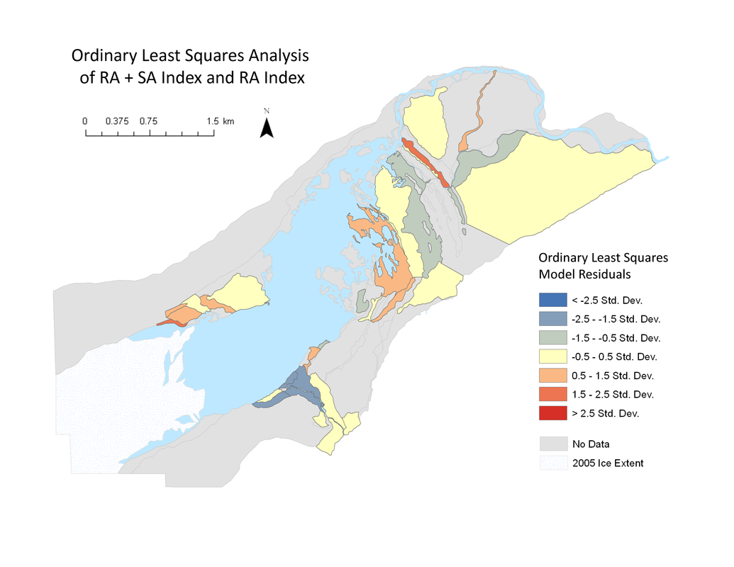
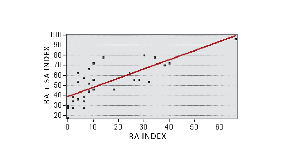
RA Index (Dependent Variable) and RA + SA Index (Response Variable)
The OLS analysis of these variables yielded the highest r-squared value and lowest P value out of all the variables examined in this study, meaning that the RA index is a good predictor of RA + SA values. On this map high residuals are found in areas where the RA + SA index value is higher than would be expected given the RA index value whereas the low residuals indicate lower RA + SA index than expected. There are two polygons with the highest residuals: one is the terminal moraine in the main valley (polygon 12A) while the other is found for one of the moraines on the north shore (polygon 1). The lowest residual values are found in several of the polygons in the South Creek tributary valley (polygons 27, 31, 32).
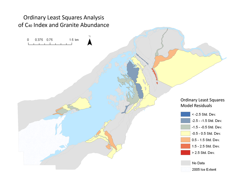
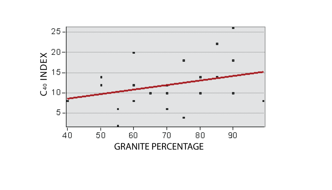
Granite Abundance (Dependent Variable) and C40 Index (Response Variable)
The OLS analysis of these two variables indicates that these two variables are significantly spatially correlated (P value = 0.0225). The polygon highest residual value, which indicates an area where the C40 index is higher than would be expected given the granite abundance value, is found within the terminal moraine complex in the main valley (polygon 12B) while other high values are found distributed across the proglacial area. The lowest residual values are found in the polygons in the main valley that are located closest to the lake (polygons 16 and 19).
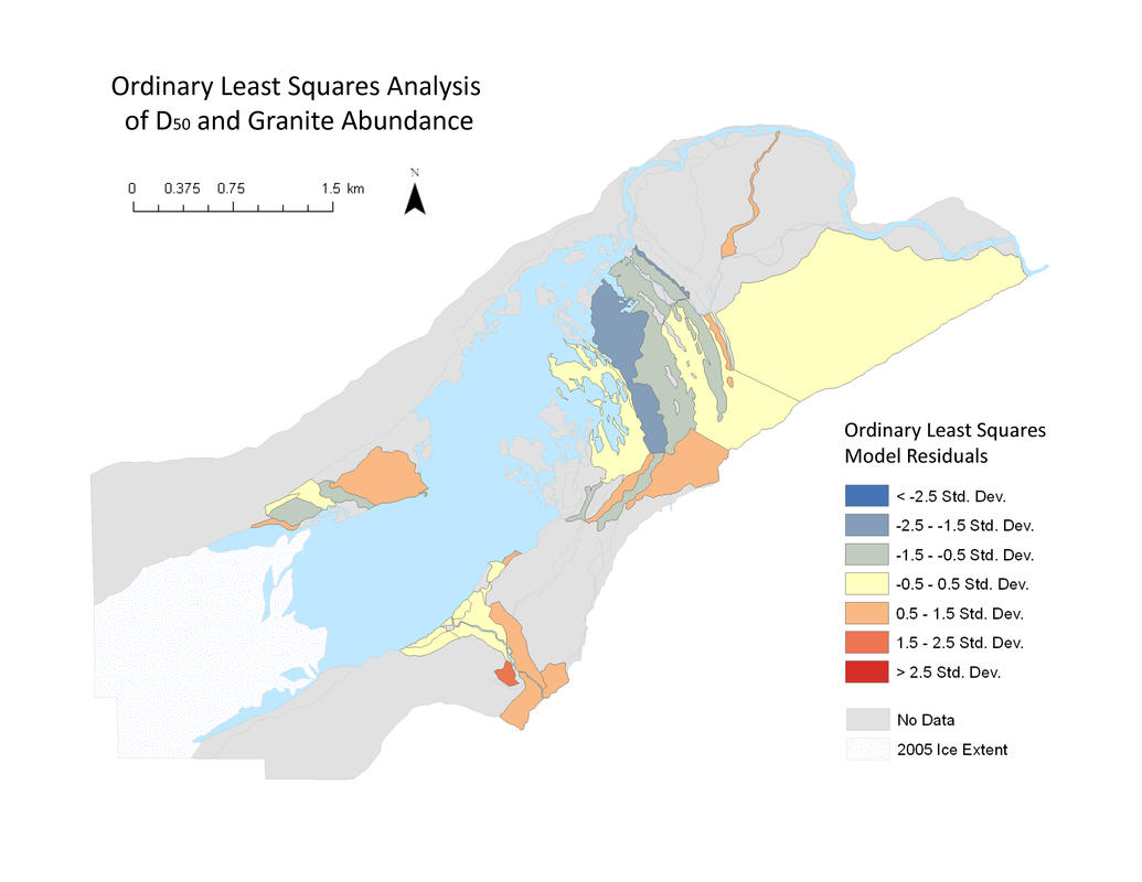
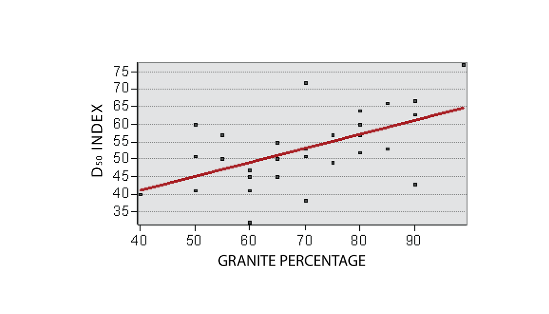
Granite Abundance (Dependent Variable) and D50 (Response Variable)
The regression analysis between these two variables found a very significant correlation (P value = 0.0002) between these two variables, although the r-squared value is not that high (0.314). On this map, the lowest residual values are primarily found in the main valley (polygons 19B has the lowest residual). These low residual values indicate that these areas have lower D50 values than predicted for the granite abundance of that given polygon. It is interesting to note that the both of the analyses using granite abundance as the dependent variable found that polygon 19B had the lowest residual value. This may indicate that instead of that polygon having lower than expected response variable values, the granite abundance value for this polygon may be exceptionally high. There are several areas that had higher than expected D50 values were found in the South Creek tributary valley (polygons 28 and 34), although high residual values were also found in some areas of the north shore and the main valley.
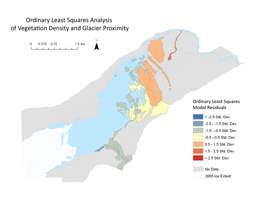
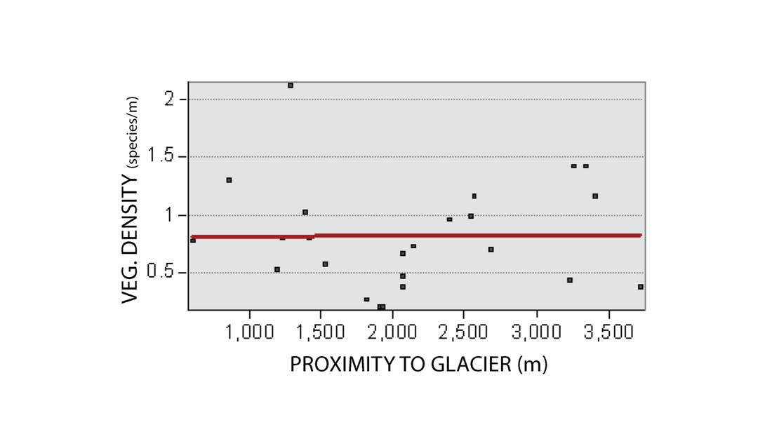
Proximity to Glacier (Dependent Variable) and Vegetation Density (Response Variable)
The analysis of these two variables was done in order to examine the effects of conducting a OLS analysis on spatially autocorrelated variables. One of the criteria of OLS analyses is that neither of the variables should be spatially autocorrelated. As both of these variables are clustered (ie. significantly spatially autocorrelated) neither of them should be used as variables in an OLS analysis. It can be seen that this is true by the fact that the resulting residual map basically just shows the a pattern which mimics the distribution of the dependent variablee and by the fact that the r-squared value is extremely low while the P value indicates that the results are not significant.
The OLS analysis of these variables yielded the highest r-squared value and lowest P value out of all the variables examined in this study, meaning that the RA index is a good predictor of RA + SA values. On this map high residuals are found in areas where the RA + SA index value is higher than would be expected given the RA index value whereas the low residuals indicate lower RA + SA index than expected. There are two polygons with the highest residuals: one is the terminal moraine in the main valley (polygon 12A) while the other is found for one of the moraines on the north shore (polygon 1). The lowest residual values are found in several of the polygons in the South Creek tributary valley (polygons 27, 31, 32).
Granite Abundance (Dependent Variable) and C40 Index (Response Variable)
The OLS analysis of these two variables indicates that these two variables are significantly spatially correlated (P value = 0.0225). The polygon highest residual value, which indicates an area where the C40 index is higher than would be expected given the granite abundance value, is found within the terminal moraine complex in the main valley (polygon 12B) while other high values are found distributed across the proglacial area. The lowest residual values are found in the polygons in the main valley that are located closest to the lake (polygons 16 and 19).
Granite Abundance (Dependent Variable) and D50 (Response Variable)
The regression analysis between these two variables found a very significant correlation (P value = 0.0002) between these two variables, although the r-squared value is not that high (0.314). On this map, the lowest residual values are primarily found in the main valley (polygons 19B has the lowest residual). These low residual values indicate that these areas have lower D50 values than predicted for the granite abundance of that given polygon. It is interesting to note that the both of the analyses using granite abundance as the dependent variable found that polygon 19B had the lowest residual value. This may indicate that instead of that polygon having lower than expected response variable values, the granite abundance value for this polygon may be exceptionally high. There are several areas that had higher than expected D50 values were found in the South Creek tributary valley (polygons 28 and 34), although high residual values were also found in some areas of the north shore and the main valley.
Proximity to Glacier (Dependent Variable) and Vegetation Density (Response Variable)
The analysis of these two variables was done in order to examine the effects of conducting a OLS analysis on spatially autocorrelated variables. One of the criteria of OLS analyses is that neither of the variables should be spatially autocorrelated. As both of these variables are clustered (ie. significantly spatially autocorrelated) neither of them should be used as variables in an OLS analysis. It can be seen that this is true by the fact that the resulting residual map basically just shows the a pattern which mimics the distribution of the dependent variablee and by the fact that the r-squared value is extremely low while the P value indicates that the results are not significant.