Spatial Distributions
Deposit Types
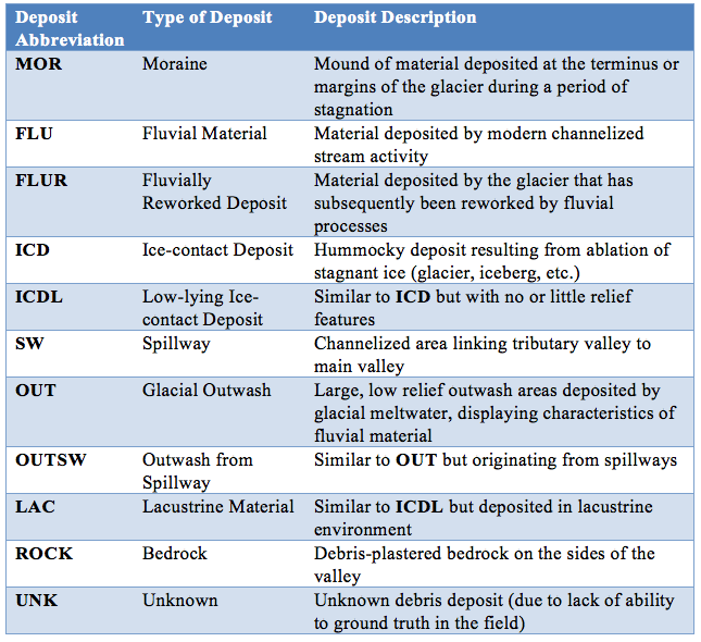
Table 4. Descriptions of deposit types
abbreviated in Fig. 2
The distribution of deposit types in the proglacial areas of Bridge Glacier were classified – shown in Fig. 4 – based on air photo interpretation and field observations. The delineation of deposits based on air photos used differences in colour, texture, and morphology to differentiate between deposit types, for example, fluvial deposits could be distinguished due to their uniform colour, lack of relief, and the presence of channels. These preliminary deposit type assignments based on air photo interpretation were then ground truthed during field expeditions in order to accurately categorize the types of deposits. Deposits that were not accessed during field work were left as UNK (or unknown) due to the uncertainty that is associated with only using air photo interpretation.
A visual inspection of the distribution map of deposit types reveals several distinct features and landform assemblages in the Bridge Glacier's proglacial area. The areas of outwash from spillways are clearly connected to the three spillways that link the South Creek tributary valley to the main valley. The largest area of outwash is linked to the southernmost spillway channel, which is consistent with the fact that this spillway drained the largest of the lake basins, whereas the outwash associated with the most northern spillway is quite minimal, as it is largely covered (presumably) by the proglacial lake.
The large terminal moraine complex located in the northeast of the outwash plain is associated with the maximal Holocene ice extent of Bridge Glacier, which occurred during the Little Ice Age (LIA) approximately 600 to 400 years BP (Ryder and Thompson, 1986; Ryder, 1991; Allen and Smith, 2007). The series of tightly packed end moraines indicates that during that period there were short durations of retreat inter-spliced with longer periods of stagnation, during which, the moraines were deposited. Between the terminal moraine complex and the ice terminus there are the remnants of two end moraines, which likely symbolized periods of glacier terminus stagnation. Of these two, the moraine closest to the ice margin is primarily only visible on the north side, likely due to the fact that the lake covers the rest of it. Areas of ICD seem to be associated with the ice stagnation that occurred when the moraines were laid down, as they are situated in the areas behind (closer to the glacier terminus) each of the moraines. The high variability of deposits around the glacial lake give an indication of the complicated effects that the lake has on the surrounding deposits. This is due to seasonal and annual changes in its water level, its leveling effect on deposits, and its sedimentation regime.
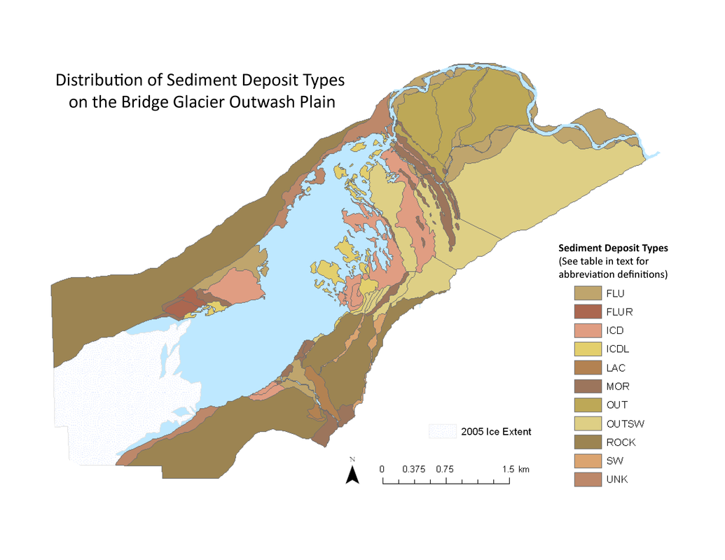
Figure 4. Distribution of sediment deposit types. See table 4 for the description of deposit type abbreviations
Clast Form Indices
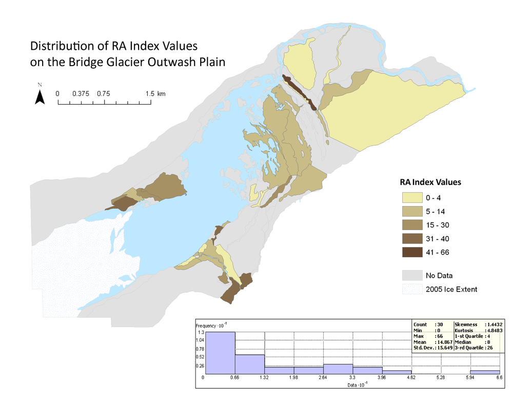
It can be seen from the map, as well as the histogram, that lower RA values are much more common in the proglacial area. The relatively high mean value (RA Index = 15.1) is likely due to the fact that there is an outlier with a high RA index value (RA Index = 66). When comparing the distribution of RA index values to the deposit distribution map, areas with the highest RA indexes are generally classified as moraines (polygons 1, 12A, 30, 34), whereas the areas with the lowest RA values are outwash deposits – both glacial and spillway (polygons 14 and 19), and lacustrine deposits (polygon 28A). Compared to the rest of the proglacial area, deposits located on the south shore of the lake seem to have overall higher RA index values.
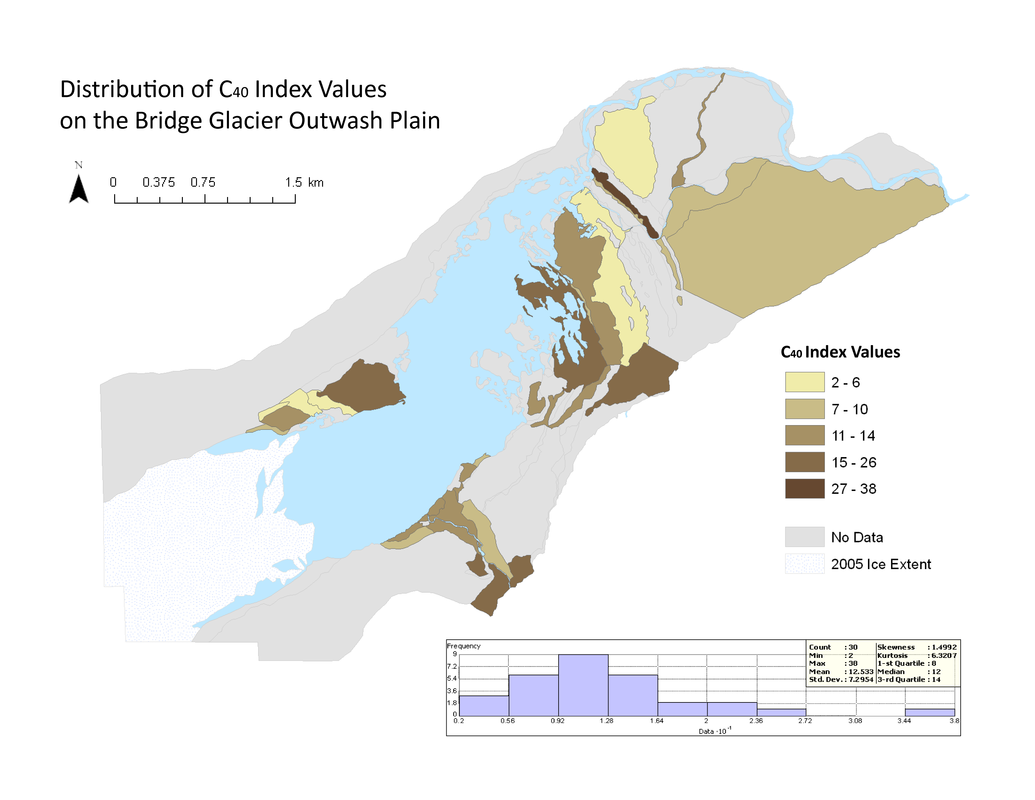
Unlike the RA index values, the C40 index values follow a more normal distribution (visible on the histogram). However, similar to the RA index value distribution, there is an outlier with a relatively high C40 index value (38). Most of the polygons have moderate C40 index values and there is less of a visible spatial distribution pattern between the deposits. The highest value is found for the terminal moraine in the main valley, while the lowest values are found in both the main valley and on the north shore (polygons 3,4,5, and 20).
Comparing the two, it is possible to see that the polygons that have the highest RA index values correspond to those that have the highest C40 index values (the terminal moraine on the main outwash apron), while the same is true for the lowest RA and C40 index values (the area of outwash directly northeast of the terminal moraine). Less of a distinct correlation is visible for the more moderate values of the two indices, indicating that a more sophisticated analysis of correlation is necessary to understand the spatial relationship between these two variables.
Clast Size
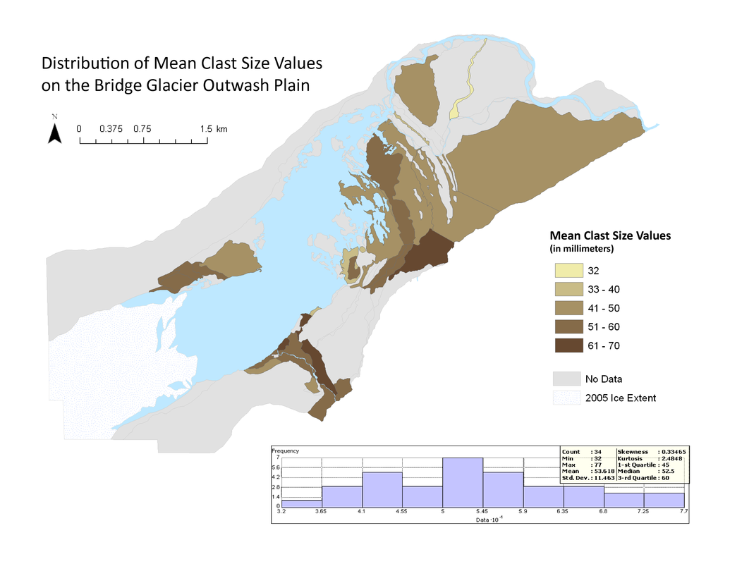
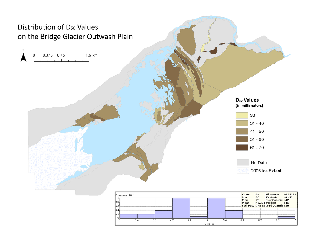
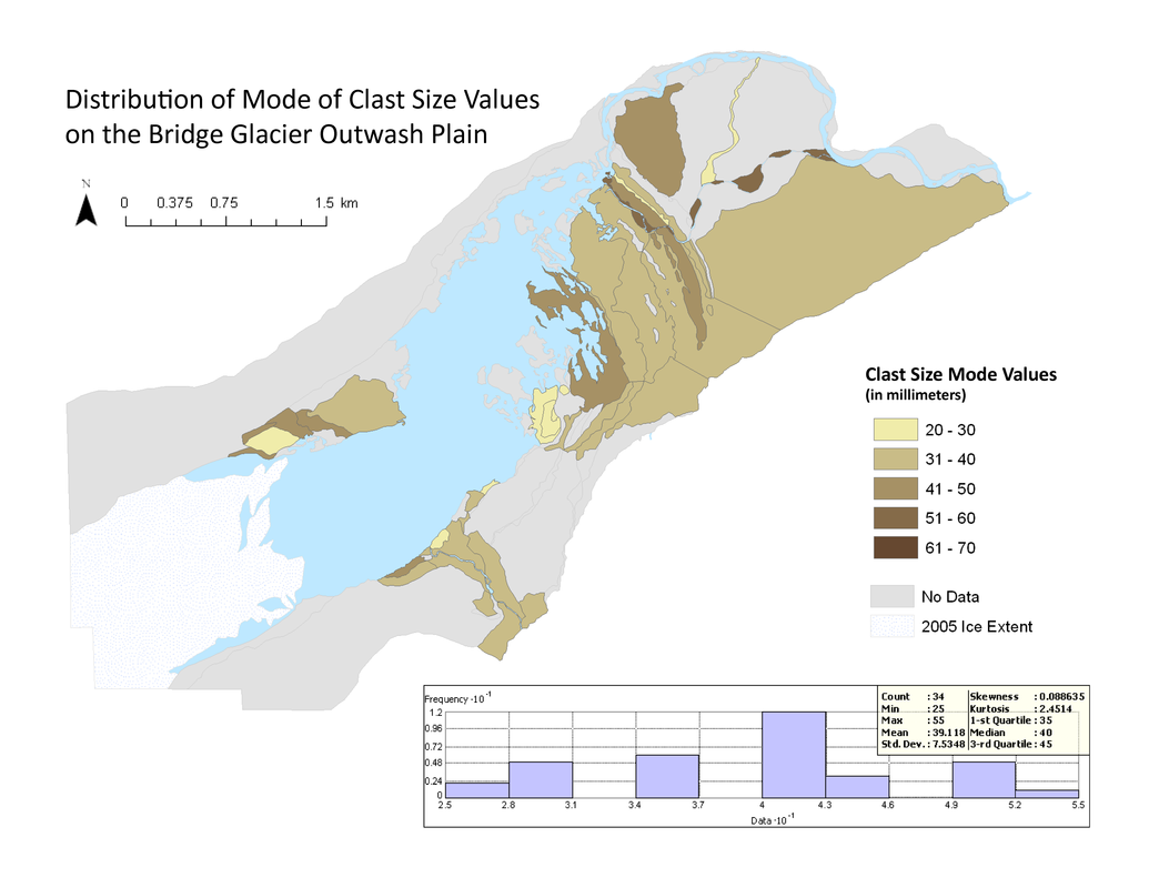
The D50 (median), mean and mode – calculated based on the data collected in the field – are beneficial to compare as they are all measures of central tendency that do not all necessarily find the same values for a given deposit. Between these three, the distribution of mean clast sizes has the highest mean value for the sampling distribution (53.6 mm) and the widest range. The distribution of mode values has the lowest mean (39.1 mm) and the smallest range. The mean clast size map generally has the highest overall values across the entire proglacial area; the D50 map has the most variation; the mode map generally has the lowest values. On the mean and D50 maps, the main outwash plain –the one that is linked to the northernmost spillway channel – displays much larger clast size values right near the mouth of the spillway compared to further away.
Due to the differences between these three maps, it is hard to say which areas have the highest proportion of large clasts. If the D50 values are taken as the best representation of the clast size distributions of each of the deposits, the highest value is found for a modern fluvial deposit (polygon 21), while the lowest value is found for an abandoned stream channel that runs through one of the glacial outwash deposits (polygon 13).
Due to the differences between these three maps, it is hard to say which areas have the highest proportion of large clasts. If the D50 values are taken as the best representation of the clast size distributions of each of the deposits, the highest value is found for a modern fluvial deposit (polygon 21), while the lowest value is found for an abandoned stream channel that runs through one of the glacial outwash deposits (polygon 13).
Clast to Matrix Composition
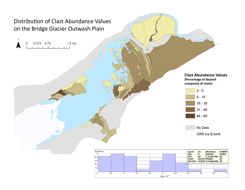
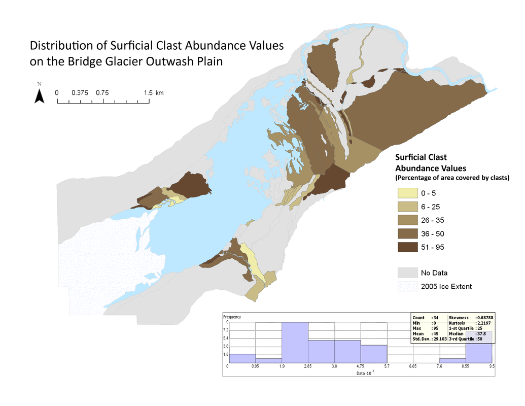
Clasts make up much more of the composition of the deposit on the surface of the deposit compared to within the deposit. This can be seen both by the fact that the surficial clast abundance values have a higher mean than that found within the deposit, and that the surficial clast abundance values are generally higher across the proglacial areas. By visual comparison, it can be seen that the areas that have higher surficial clast abundance values correspond to areas with high clast values within the deposit (such as near the mouth of the southernmost spillway), although this is not always the case (such as for the northermost OUT deposit). While most of the polygons have some proportion of clasts present on the surface, there are many polygons that have very low or non-existant clast components within the deposits. Also, neither of the distributions follow a normal distribution, both seem to have a bimodal distribution. The areas with the highest clast abundance values for both the surficial and within-deposit variables are at the mouth of the main spillway (polygon 19A proximal) and the moraines on the north shore (polygons 1 and 3), while the area with the lowest values for both is the lacustrine deposit in the South Creek tributary valley (polygon 28A).
Other Variables
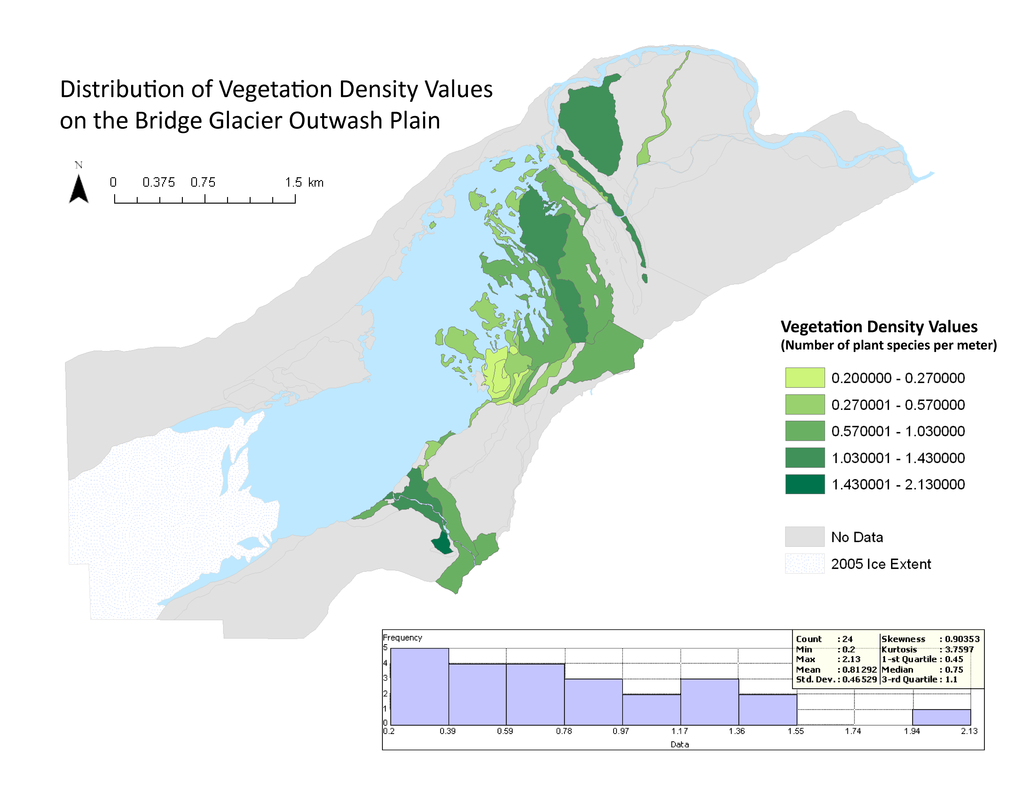
Vegetation density is the highest in areas that are further from the lake. The highest vegetation density is found on the lacustrine deposits in the South Creek tributary valley (polygon 28B). The lowest value is found on the ICD nearest to the ice terminus in the main valley (polygons 16A and 16B).
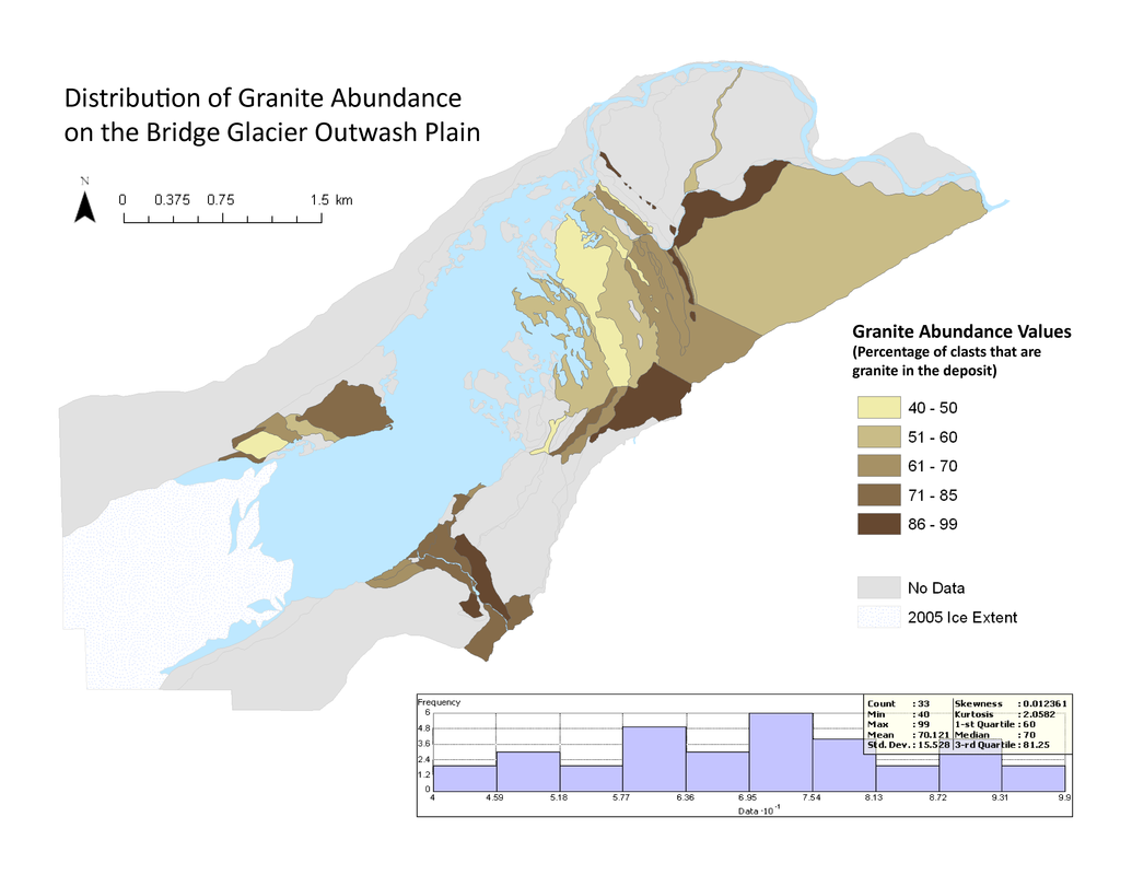
On the main outwash plain that is linked to the northernmost spillway, granite abundances decrease with distance from the mouth of the spillway. Granite abundances are also quite high for all of the deposits in the South Creek tributary valley (especially polygons 28A and 28B), possibly due to the fact that rock within that area may be coming from bedrock sources where granite is more common. The lowest values are found within most of the morainal deposits (polygons 11A, 12E, 15B), as well as part of the spillway outwash (polygon 19B), in the main valley and in the fluvially reworked deposits on the north shore (polygon 2).
On the main outwash plain that is linked to the northernmost spillway, granite abundances decrease with distance from the mouth of the spillway. Granite abundances are also quite high for all of the deposits in the South Creek tributary valley (especially polygons 28A and 28B), possibly due to the fact that rock within that area may be coming from bedrock sources where granite is more common. The lowest values are found within most of the morainal deposits (polygons 11A, 12E, 15B), as well as part of the spillway outwash (polygon 19B), in the main valley and in the fluvially reworked deposits on the north shore (polygon 2).